Text Analysis of The Lizzie Bennet Diaries
Inspired by Julia’s Silge’s recent talk on Tidytext as part of NASA Datanauts, and her blog posts, I decided to try my hand at some text analysis. Julia’s examples focus on the works of Jane Austen. As Jane Austen has been adapted so many time, I decided to “adapt” Julia’s talk for the modern works of Austen’s book Pride and Prejudice - specifically the Lizzie Bennet Diaries.
 Image source: Pemberly Digital
The Lizzie Bennet Diaries
The Lizzie Bennet Diaries is a modern adaptation of Jane Austen’s Pride and Prejudice for YouTube. The story is told through a series of Vlogs by Lizzie Bennet as part of a school project. The series, created by Hank Green and Bernie Su, first aired on April 9, 2012, making this year the 5th Anniversary of the series! Altogether, the series filmed more than 100 video episodes with over 9.5 hours of video making it the longest adaption of Pride and Prejudice to date.
Along with the main LBD channel, there are also some supporting channels. These allow other characters to tell parts of the story that Lizzie doesn’t take part in. For example, Lydia’s Vlogs include the story on how she meets George Wickham and their budding relationship. While not required viewing, these extra videos help round out the experience.
Since the series ended, 2 books have come out from the creators and writers of the original videos: one that follows the videos but adds some more detail to Lizzie’s life, and one that focuses on Lydia’s story after the series ends.
In honor of LBD’s 5th Anniversary, let’s do some LBD text analysis! Happy Anniversary LBD!

Analysis
Gathering Data
The first part of this analysis is grabbing all the text from YouTube.
To access the API, I use the tuber
package by Gaurav Sood.
library(tidyverse)
library(tuber)

yt_oauth(app_id, app_password)
The fist step was to find the channel id to access the LBD playlist. I
do a quick search for lizziebennet to find some videos that I know are
part of the series.
search <- yt_search("lizziebennet")[1:5, ]
search %>% select(title, channelId)

##                                                       title
## 1                         My Name is Lizzie Bennet  - Ep: 1
## 2 The Lizzie Bennet Diaries - Episódio 98 (LEGENDADO PT-BR)
## 3                                      Yeah I Know - Ep: 61
## 4                                 Introducing Lizzie Bennet
## 5                                  The Lizzie Trap - Ep: 78
##                  channelId
## 1 UCXfbQAimgtbk4RAUHtIAUww
## 2 UCfhdE-vIhW9GD0eGdd300ag
## 3 UCXfbQAimgtbk4RAUHtIAUww
## 4 UCGaVdbSav8xWuFWTadK6loA
## 5 UCXfbQAimgtbk4RAUHtIAUww
With the channel ID in hand, I can now access the channel’s resources to
find the playlist ID, which I will use to access all the videos in that
playlist. list_channel_resources for tuber creates a list of channel
attributes and buried in that list in the playlist ID.
# Channel Information
a <- list_channel_resources(filter = c(channel_id="UCXfbQAimgtbk4RAUHtIAUww"), part="contentDetails")

# Uploaded playlists:
playlist_id <- a$items[[1]]$contentDetails$relatedPlaylists$uploads

playlist_id

## [1] "UUXfbQAimgtbk4RAUHtIAUww"
The YouTube API automatically pages videos so the max you get per page is
- I know I need more than that, so I created a function that I call a few times to get all the videos. (This way works, but I would love any comments on how to make it better.)
# pass NA as next page to get first page
nextPageToken <- NA
vid_info <-{}

# Loop over every available page
repeat {
  vids <- get_playlist_items(filter= c(playlist_id=playlist_id), page_token = nextPageToken)
  vid_ids <- map(vids$items, "contentDetails") %>%
      map("videoId")  %>%
      unlist()

  vid_info <- vid_info %>% bind_rows(tibble(ids = vid_ids))

  # get the token for the next page
  nextPageToken <- ifelse(!is.null(vids$nextPageToken), vids$nextPageToken, NA)

  # if no more pages then done
  if(is.na(nextPageToken)){
     break
  }

}

# check that I have all 112 videos
nrow(vid_info)

## [1] 112
Now that I have a list of video IDs, I can use get_captions to access
the text of the videos. I also use xmlTreeParse and xmlToList to
covert the caption into into an easily accessible lines of text. I put
the text, video ID, and video title in a tibble for use in tidydata.
library(XML)

getText <- function(id){
  x <- get_captions(id, lang = "en")
  title <- get_video_details(id)$title
  a <- xmlTreeParse(x)
  text <- a$doc$children$transcript
  text <- xmlToList(text, simplify = TRUE, addAttributes = FALSE) %>%
    tibble() %>%
    mutate(id = id, title = title)
  return(text)
}

text <- map_df(vid_ids, getText) %>%
  set_names(c("text", "vid_id", "title"))
I don’t actually want to refer to each video by it’s full title, so I do some data munching to get each episode’s number (1-100). Notice, the Q&A videos do not get a episode number assigned to them. For the sake of this analysis, I’ve decided to only work with the main 100 episodes.
titles <- text %>%
  distinct(title) %>%
  mutate(title = ifelse(title == "Question and Answers #3 (ft. Caroline Lee)", "Questions and Answers #3 (ft. Caroline Lee)", title),
         ep_num = gsub("[- .)(+!',/]|[a-zA-Z]*:?","", title),
         ep_num = ifelse(title == "2 + 1 - Ep: 73", 73, ep_num),
         ep_num = ifelse(title == "25 Douchebags and a Gentleman - Ep:18", 18, ep_num),
         ep_num = ifelse(title == "Bing Lee and His 500 Teenage Prostitutes - Ep: 4", 4, ep_num),
         ep_num = parse_number(ep.num)
         ) %>%
  filter(!grepl("Questions and Answers", title)) %>%
  arrange(ep_num)
One of the problems with using captions, is the messy text. I used a
simple set of gsub commands to transform obvious punctuation marks into their
English counterparts. I also pulled out the character SPEAKING the words
from the text itself. I left this column alone in the data set, but might
one day go back and focus an analysis on speaking characters.
library(tidytext)
library(stringr)
lizziebennet <- text %>%
left_join(titles, by="title") %>%
filter(!is.na(ep_num)) %>%
arrange(ep_num) %>%
mutate(linenumber = row_number()) %>%
mutate(text = gsub("'", "'", text),
text = gsub(""", '\"', text),
text = gsub("&", "and", text),
character = str_extract(text, "^[a-zA-Z]*:"),
text = sub("^[a-zA-Z]*:", "", text)
) %>%
arrange(ep_num, linenumber)
Okay, so now the text is mostly in place. The first thing I did was look at word counts. The most common words are not surprising, it’s just a list of the characters.
lizziebennet %>%
  tidytext::unnest_tokens(word, text) %>%
  anti_join(stop_words, by="word") %>%
  count(word, sort=TRUE) %>%
  top_n(10)

## # A tibble: 10 × 2
##         word     n
##        <chr> <int>
## 1     lizzie   460
## 2       jane   301
## 3      darcy   243
## 4       bing   232
## 5    collins   220
## 6      lydia   196
## 7     bennet   194
## 8  charlotte   180
## 9       yeah   178
## 10      time   176
Not surprisingly, the most common trigrams are from the phrase that begins every episode, “My name is Lizzie Bennet and…”
lizziebennet %>%
  tidytext::unnest_tokens(word, text, token="ngrams", n=3) %>%
  count(word, sort=TRUE) %>%
  top_n(10)

## # A tibble: 10 × 2
##                 word     n
##                <chr> <int>
## 1         my name is   106
## 2   is lizzie bennet    96
## 3     name is lizzie    96
## 4  lizzie bennet and    84
## 5       i don't know    40
## 6          oh my god    36
## 7           a lot of    33
## 8        going to be    31
## 9       what are you    29
## 10     mr collins oh    28
I was also especially amused by So good to see you! and THE MOST AWKWARD DANCE EVER being in the Top 10 5-grams.
## # A tibble: 12 × 2
##                           word     n
##                          <chr> <int>
## 1     my name is lizzie bennet    95
## 2    name is lizzie bennet and    83
## 3       is lizzie bennet and i    19
## 4    is lizzie bennet and this    14
## 5    lizzie bennet and this is    11
## 6           so good to see you     9
## 7       had nothing to do with     5
## 8     is lizzie bennet and i'm     5
## 9       lizzie bennet and i am     5
## 10 the most awkward dance ever     5
## 11     what are you doing here     5
Sentiment Analysis
I’ve chosen to use the Bing lexicon (because of Bing Lee, get it?). In Tidydata, sentiment analysis is easy because you just join the lexicon against your tokenzied words.
bing <- sentiments %>%
        filter(lexicon == "bing") %>%
        select(-score)

lbwordcount <- lizziebennet %>%
  tidytext::unnest_tokens(word, text) %>%
  anti_join(stop_words) %>%
  count(title)

lbsentiment <- lizziebennet %>%
  tidytext::unnest_tokens(word, text) %>%
  anti_join(stop_words) %>%
  inner_join(bing) %>%
  count(title, index=ep_num, sentiment) %>%
  spread(sentiment, n, fill = 0) %>%
  left_join(lbwordcount) %>%
  mutate(sentiment = positive - negative,
         sentiment = sentiment / n)
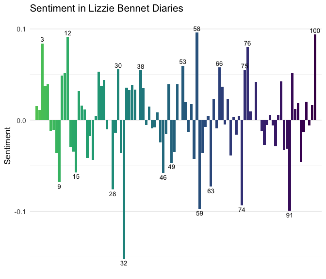
Most positive sentiment episodes:
## # A tibble: 5 × 2
##                                       title  sentiment
##                                       <chr>      <dbl>
## 1                    Care Packages - Ep: 58 0.09623431
## 2                         The End - Ep: 100 0.09375000
## 3                   Jane Chimes In - Ep: 12 0.09132420
## 4 My Parents: Opposingly Supportive - Ep: 3 0.08415842
## 5      Wishing Something Universal - Ep: 76 0.08018868
Most negative sentiment episodes:
## # A tibble: 5 × 2
##                            title   sentiment
##                            <chr>       <dbl>
## 1   Turn About the Room - Ep: 32 -0.15217391
## 2        How About That - Ep: 91 -0.09937888
## 3          Staff Spirit - Ep: 59 -0.09745763
## 4 How to Hold a Grudge  - Ep: 74 -0.09352518
## 5      Meeting Bing Lee - Ep: 28 -0.07614213
The next step was to visualize this in a way where you can look at the sentiment over the episodes.
library(viridis)
theme_set(theme_bw()) # a theme with a white background

ggplot(lbsentiment, aes(x=index, sentiment, fill=as.factor(index))) +
        geom_bar(stat = "identity", show.legend = FALSE) +
        theme_minimal(base_size = 13) +
        geom_text(data=plot_text, aes(x=index, y=sentiment, label=index), size=3.5) +
        labs(title = "Sentiment in Lizzie Bennet Diaries",
             y = "Sentiment") +
        scale_fill_viridis(end = 0.75, discrete=TRUE, direction = -1) +
        scale_x_discrete(expand=c(0.02,0)) +
        theme(strip.text=element_text(hjust=0)) +
        theme(strip.text=element_text(face = "italic")) +
        theme(axis.title.x=element_blank()) +
        theme(axis.ticks.x=element_blank()) +
        theme(axis.text.x=element_blank())
 Sentiment by main episode of LBD.
Julia’s sentiment analysis of the original text is much more positive than my LBD analysis, with two negative portions relating to Darcy proposing to Elizabeth and Lydia running away with Wickham. I had expected a similar “Wickham” negative spike in this plot, and while the section of Wickham related episodes (Ep 84 to Ep 89) is surely negative it’s not more negative than some of the introductory episodes.
One could argue, that since most of the Lydia - Wickham story line happens off screen and in Lydia’s blogs, that would explain that lack of a clear negative spike in the Wickham episodes.
More sentiment
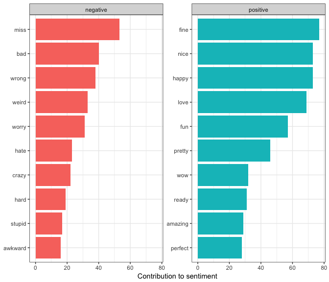
Continuing the analysis, I wanted to look at which words were causing the largest effect on the overall sentiment.
bing_word_counts %>%
  group_by(sentiment) %>%
  top_n(10) %>%
  mutate(word = reorder(word, n)) %>%
  ggplot(aes(word, n, fill = sentiment)) +
  geom_col(show.legend = FALSE) +
  facet_wrap(~sentiment, scales = "free_y") +
  labs(y = "Contribution to sentiment",
       x = NULL) +
  coord_flip()

Given that this is a modern adaption, it’s interesting that much like the analysis done on the original “miss” is the top contribution to negative sentiment. In the original text I would assume a higher count of “Miss Bennet’s” to the modernized version. However, Lizzie does talk about you she’ll miss Charlotte, or she misses her home… etc, so it’s not too surprising to see it have a considerable contribution here.
I did a bit of an investigation into this with bigrams.
lizziebennet %>%
  tidytext::unnest_tokens(bigram, text, token="ngrams", n=2) %>%
  separate(bigram, c("word1", "word2"), sep = " ") %>%
  filter(word1 == "miss") %>%
  mutate(miss_in_name = ifelse(word2 %in% c("bennet", "lu"), "Yes", "No")) %>%
  count(miss_in_name)

## # A tibble: 2 × 2
##   miss_in_name     n
##          <chr> <int>
## 1           No    26
## 2          Yes    27
And oddly enough, the use of the word “miss” is about half and half between “I miss [person/thing]” and “Miss Bennet” type phrases. Interesting! (Anyone want to guess who refers to Lizzie as Miss Bennet the most? Unsurprisingly, it’s Ricky Collins.)
More with Bigrams
bigrams_separated <- lizziebennet %>%
  tidytext::unnest_tokens(bigram, text, token="ngrams", n=2) %>%
  separate(bigram, c("word1", "word2"), sep = " ") %>%
  filter(!word1 %in% stop_words$word,
         !word2 %in% stop_words$word) %>%
  count(word1, word2, sort = TRUE)

bigrams_separated %>%
  ungroup() %>%
  top_n(10)

## # A tibble: 11 × 3
##      word1   word2     n
##      <chr>   <chr> <int>
## 1   lizzie  bennet   132
## 2     bing     lee    43
## 3   george wickham    24
## 4      hey  lizzie    24
## 5       de  bourgh    22
## 6    ricky collins    21
## 7      los angeles    20
## 8     miss  bennet    19
## 9     tour  leader    18
## 10   video    blog    17
## 11 william   darcy    17
Not surprisingly, the common bigrams are first and last names of characters, but there’s also some fun other popular bigrams with “tour leader” and “video blog.” I guess vlog wasn’t super popular to use on it’s own yet.
Network of Words
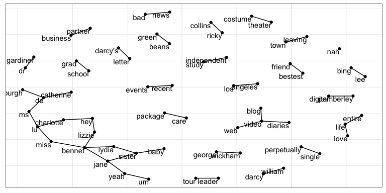
One of my favorite part of tidytext is the example on making a bigram network. It’s just so fun!
library(igraph)
library(ggraph)

set.seed(42)

bigrams_separated %>%
  filter(n > 5) %>%
  graph_from_data_frame() %>%
  ggraph(layout = "fr") +
  geom_edge_link() +
  geom_node_point() +
  geom_node_text(aes(label = name), vjust = 1, hjust = 1) +
  theme(axis.title.x=element_blank()) +
  theme(axis.ticks.x=element_blank()) +
  theme(axis.text.x=element_blank()) +
  theme(axis.title.y=element_blank()) +
  theme(axis.ticks.y=element_blank()) +
  theme(axis.text.y=element_blank())

I especially enjoy the Bennet sister cluster in the left corner.
I leave you with this last picture.
 Some of cast of Lizzie Bennet Diaries and me. Vidcon 2014